Introduction

Modeling time series data can be surprisingly complex, especially when it shows both cyclical patterns and underlying trends. What appears to be a simple upward or downward trend often masks multiple competing cycles—daily, weekly, seasonal, and irregular—that interact in unexpected ways. Add to this the difficulty of distinguishing meaningful signals from statistical noise, and the task becomes even more challenging.

A friend of mine was dealing with a similar problem — trying to fit a model to real-world isotope data. It turned into an engaging hands-on experiment for me. I found that the right mix of intuitive feature engineering and carefully selected activation functions could enable surprisingly accurate predictions. In this blog post, I'll share the approach I developed, using a basic neural network enhanced with domain-informed features to effectively model data that shows both strong cyclical behavior and clear trending characteristics.

1#Imports
2import numpy as np
3import pandas as pd
4import matplotlib.pyplot as plt
5plt.style.use('./deeplearning.mplstyle')
6import tensorflow as tf
7from tensorflow import keras
8from sklearn.preprocessing import StandardScaler

Dataset

To explore this modeling challenge, I intentionally selected an illustrative yet straightforward dataset — one that wouldn't distract me with complexity but would still capture the core of the problem. I found this dataset on Kaggle, which includes daily atmospheric CO₂ concentration measurements from January 25, 2015, to February 13, 2025, comprising a total of 3,673 data points. What makes it ideal for this experiment is that it explicitly separates the cyclical and trending components of CO₂ levels. This clear separation allowed me to focus on the main task: building a model that can learn both patterns simultaneously. As shown in the figure below, the green curve depicts the seasonal cycle. At the same time, the yellow line indicates the long-term upward trend in CO₂ concentrations—a classic example of the kind of signal I aimed to analyze using neural networks and feature engineering.

1# Load the dataset
2file_path = './co2 concentration.csv'
3df = pd.read_csv(file_path)
4df.describe()

Data Preparation

The dataset has year, month, and day as separate columns.

1# Display the first few rows of the dataset
2df.head()

The first thing I did was to combine the year, month, and day into a datetime column and use that as the index.

1# Combine year, month, and day into a single datetime column
2df['date'] = pd.to_datetime(df[['year', 'month', 'day']])
3df = df.drop(columns=['year', 'month', 'day'])
4df = df.set_index('date')
5df.head()

Next, plot the raw data to visualize its appearance.

1# Plot the CO2 cycle and trend over time
2plt.style.use('dark_background')
3plt.figure(figsize=(14, 7))
4plt.plot(df.index, df['trend'], label='Trend', color='yellow', linewidth=1.5)
5plt.plot(df.index, df['cycle'], label='Cycle', color='lime', linewidth=1.5)
6plt.grid(True, linestyle=':', alpha=0.3, linewidth=1, color='whitesmoke') 
7plt.xlabel('Date')
8plt.ylabel('CO2 Concentration')
9plt.title('CO2 Concentration Cycle and Trend Over Time')
10plt.legend()
11plt.show()

The data is clearly cyclic in nature, but also exhibits an upward trend over time. It's cyclic within the year, where CO₂ levels increase during the winter months in the northern hemisphere at the beginning of the year, but fall steadily after reaching a peak sometime in summer for the rest of the year. However, year after year, this trend continues to rise with increasing CO₂ levels.

1# Plot the CO2 cycle and trend over time
2plt.style.use('dark_background')
3df_every_third = df.iloc[::20]
4plt.figure(figsize=(14, 7))
5plt.scatter(df_every_third.index, df_every_third['cycle'], label='Cycle', color='lime', marker='.', s=7, linewidth=1.5)
6plt.grid(True, linestyle=':', alpha=0.3, linewidth=1, color='whitesmoke') 
7plt.xlabel('Date')
8plt.ylabel('CO2 Concentration')
9plt.title('CO2 Concentration Cycle and Trend Over Time')
10plt.legend()
11plt.show()

Preparing data for fitting.

My first instinct for feature engineering was to use time as the primary input feature — after all, the data is indexed by date. To keep things simple, I converted each date into an integer representing the number of days since the start of the dataset. This essentially mirrored the row index, which conveniently served as a proxy for time progression.

1# Prepare the data for modeling
2# Use the index number as the number of days from when the data is captured in the dataset. So the first date is day 0, the next date is day 1 etc.
3X = df.index.factorize()[0].reshape(-1, 1)  # Use date as the feature
4y = df['cycle'].values  # Use trend as the target

Feature Normalization

I then reshaped this index into a 2D array to make it compatible with the neural network input. Since the raw index values ranged into the thousands (over 3,600 days), I applied normalization to scale the feature. Neural networks tend to learn more effectively when input features are within a compact range — typically between 0 and 1 — as large ranges can lead to unstable gradients or slower convergence during training.

1# its best to normalize this feature, number of days, as the range is too large.
2X_mean = X.mean()
3X_std = X.std()
4X_norm = (X - X_mean)/X_std
5
6print(f"Peak to Peak range in Raw        X:{np.ptp(X,axis=0)}")   
7print(f"Peak to Peak range in Normalized X:{np.ptp(X_norm,axis=0)}")

Starting Simple: Baseline Neural Network Architecture

For my initial experiment, I began with a deliberately simple neural network architecture to maintain focus on understanding the data dynamics. The model consisted of a single hidden layer with 4 neurons, utilizing a ReLU activation function, followed by an output layer with a single neuron and linear activation. This minimalist setup served as a baseline to test whether even a small network, when paired with the right features, could effectively learn both the cyclic and trending components of the CO₂ data.

1# Define the model model
2model = tf.keras.Sequential([
3    tf.keras.layers.Dense(4, activation='relu', input_shape=(1,)),
4    tf.keras.layers.Dense(1, activation='linear')
5])
6
7# Compile the model
8model.compile(optimizer='adam', loss='mean_squared_error')
9model.summary()

I chose the ReLU (Rectified Linear Unit) activation function for the hidden layer because it’s simple, computationally efficient, and highly effective at introducing non-linearity into the model. ReLU activates only when the input is positive, which helps the network learn complex patterns — such as those found in cyclic data — without suffering from the vanishing gradient problem that can slow down or stall training with other functions like sigmoid or tanh. Both sigmoid and tanh compress their outputs into narrow ranges (between 0 and 1 and -1 and 1, respectively), which can limit their ability to model larger variations or subtle differences in data unless they are carefully normalized.

For the output layer, I used a linear activation function because the goal is to predict CO₂ concentration values, which are real-valued, unbounded, and continuous. A linear activation outputs any real number, unlike sigmoid or tanh, which would squash predictions into a fixed range, making them unsuitable for regression tasks like this. Linear activation ensures that the model isn’t artificially restricting the output range, which is critical when tracking upward trends or larger seasonal swings in the data.

Training the model

Next, I trained the model using the Kaggle data provided. This basic time-based feature was surprisingly effective when paired with even a minimal neural network. It captured the general upward trend in CO₂ levels, although it still struggled with the finer cyclical details, which I addressed next with more targeted features.

1# Train the model
2model.fit(X_norm, y, epochs=1000, verbose=1)
3
4# Get the learned weights
5weights_0, bias_0 = model.layers[0].get_weights()
6print(f"Learned weight: {weights_0}, bias: {bias_0}")
7
8weights_1, bias_1 = model.layers[1].get_weights()
9print(f"Learned weight: {weights_1}, bias: {bias_1}")

With the basic model in place and the normalized time-based feature as input, I trained the network for 1,000 epochs. This provided the model with sufficient opportunity to learn the underlying trend in the data using the simple architecture. Once training was complete, I used the learned weights and biases to generate predictions across the entire dataset.

1# Make predictions based on the Weights and biases after training the simple model.
2y_pred = model.predict(X_norm)
3

To visually evaluate the model’s performance, I plotted the predicted values alongside the original data. As shown in the figure below, the predicted curve (in red) closely follows the long-term trend of the CO₂ concentrations, capturing the upward movement effectively, though it doesn't yet account for the seasonal cycles. This initial result validated that even a minimalist setup, when fed the right feature, could approximate the trend component of the time series reasonably well.

1# Plot the CO2 cycle and trend over time
2plt.figure(figsize=(14, 7))
3plt.plot(df.index, df['cycle'], label='Cycle', color='lime', linewidth=1.5)
4plt.plot(df.index, y_pred, label='PredFull', color='red', linewidth=1.5)
5plt.grid(True, linestyle=':', alpha=0.4) 
6
7plt.xlabel('Date')
8plt.ylabel('CO2 Concentration')
9plt.title('CO2 Concentration Cycle and Trend Over Time')
10plt.legend()
11plt.show()

Teaching the Model to Recognize Cycles

While the simple model did a decent job of capturing the overall upward trend, it clearly missed the cyclical patterns — the seasonal rises and dips that repeat year after year. This was expected, since the model had only seen time as a linear input, which isn’t well-suited to representing repeating or periodic behavior. To address this, I turned to a classic technique: sinusoidal feature engineering.

I used the day of the year as a feature, since CO₂ concentrations tend to follow seasonal rhythms. To do this, I first created a timestamp column from the original date field, allowing me to extract the day of the year numerically. I then transformed this into two new features using sine and cosine functions, effectively mapping the time of year onto a circle. These sinusoidal features give the model a sense of periodicity, helping it recognize where it is in the annual cycle and making it easier for the neural network to detect and model seasonal fluctuations.

1# Make a copy of the original dataset.
2new_df = df.copy()
3new_df['timestamp_s'] = new_df.index.map(pd.Timestamp.timestamp)

To convert a day into Sine and Cosine components, I used the number of seconds in a day and converted the timestamp in seconds into the number of days. Then, I found the sine value of that, treating it as radians. After that, we normalize the Sine and Cosine components.

1# Use number of seconds in a day to convert timestamp to number of days from epoch.
2day = 24*60*60
3
4# Find sine and cosine of number of days
5new_df['day_sin'] = np.sin(new_df['timestamp_s'] * (2 * np.pi / day))
6new_df['day_cos'] = np.cos(new_df['timestamp_s'] * (2 * np.pi / day))
7
8# Normalize the sine and cosine component
9s_mean = new_df['day_sin'].mean()
10s_std = new_df['day_sin'].std()
11
12c_mean = new_df['day_cos'].mean()
13c_std = new_df['day_cos'].std()
14
15new_df['day_sin_norm'] = (new_df['day_sin'] - s_mean)/(s_std + 1e-8)
16new_df['day_cos_norm'] = (new_df['day_cos'] - c_mean)/(c_std + 1e-8)
17
18new_df.head()

Same Model, Smarter Inputs

To incorporate the newly engineered sinusoidal features, I created a second model with a similar architecture to the first. This time, instead of a single input (the normalized time index), the model takes in two features: the sine and cosine components derived from the day of the year. The architecture remains intentionally simple — it consists of just one hidden layer with 4 neurons and a ReLU activation, followed by an output layer with a single neuron using linear activation. This setup allows the model to process both cyclical signals together and learn how they contribute to the overall pattern in the data. By feeding the network more informative and seasonally aware input, I hoped it would now be able to model not just the trend, but also the recurring seasonal fluctuations more accurately.

1number_of_features=2
2# Create a mew model that takes these two new features as input
3model_2 = tf.keras.Sequential([
4    tf.keras.layers.Dense(4, activation='relu', input_shape=(number_of_features,)),
5    tf.keras.layers.Dense(1, activation='linear')
6])
7
8# Compile the model
9model_2.compile(optimizer='adam', loss='mean_squared_error')
10model_2.summary()

Prepare data for the new model

Next, I prepared the input data for the new model using the sine and cosine columns derived from the day of the year. These two features were extracted from the dataframe and combined into a 2D input array. With the data ready, I retrained the model using the same architecture — one hidden layer with 4 ReLU neurons feeding into a linear output. This time, the network had the tools it needed to learn the underlying seasonal patterns in the data.

1# Prepare data
2# Select specific columns and convert to array
3selected_columns = ['day_sin_norm', 'day_cos_norm']
4X_sin_cos_days = new_df[selected_columns].values
5y_train = new_df['cycle'].values
6print (f"Input Shape: {X_sin_cos_days.shape}, output shape: {y_train.shape}")

Train the model

1# Train the model
2model_2.fit(X_sin_cos_days, y_train, epochs=1000, verbose=0)
3
4# Get the learned weights
5weights_0, bias_0 = model_2.layers[0].get_weights()
6print(f"Learned weight: {weights_0}, bias: {bias_0}")
7
8weights_1, bias_1 = model_2.layers[1].get_weights()
9print(f"Learned weight: {weights_1}, bias: {bias_1}")

1def plot_predictions(predictions, label):
2    # Plot the CO2 cycle and trend over time
3    plt.figure(figsize=(14, 7))
4    plt.plot(df.index, df['cycle'], label='Actual CO2 Concentration', color='lime', linewidth=1.5)
5    plt.plot(df.index, df['trend'], label='Trend', color='yellow', linewidth=1.5)
6    plt.plot(df.index, predictions, label=label, color='red', linewidth=2.5)
7    plt.grid(True, linestyle=':', alpha=0.5, linewidth=1, color='whitesmoke') 
8
9    plt.xlabel('Date')
10    plt.ylabel('CO2 Concentration')
11    plt.title('CO2 Concentration Cycle and Trend Over Time')
12    plt.legend()
13    plt.show() 

1y_pred = model_2.predict(X_sin_cos_days)
2plot_predictions(y_pred, 'Predicted using sin and cos of days as features')

After training this updated model with sine and cosine features, I generated predictions and visualized the results. As seen in the plot, the red line represents the model’s predictions. While the model did begin to capture the cyclical nature of the CO₂ data, it fell short in two key areas: the amplitude and frequency of the cycles are off, and it appears to have completely ignored the upward trend. This isn't entirely surprising — the model was only fed information about seasonality (via the sine and cosine of the day), without any knowledge of how the values change over time. I decided to address the trend later, focusing solely on making the model learn the cyclic trend as accurately as possible.

But before we tackle that, I wanted to explore whether a slightly deeper architecture could improve the model's ability to match the shape of the cycle. So, I experimented by adding a second hidden layer with two neurons and ReLU activation, while keeping the original hidden layer of 4 neurons intact. This slight increase in depth might allow the network to learn more nuanced relationships between the sine/cosine inputs and the target signal, potentially helping it better model the shape and timing of the cycles.

Refining the Architecture: Adding Depth to the Network

At this point, I began experimenting more freely with the neural network architecture. Since the previous model using sine and cosine inputs had begun to recognize the cyclical structure in the data — though imperfectly — I wondered whether increasing the model's depth could help it better capture the amplitude and frequency of the cycles.

To test this, I added an additional hidden layer with 2 neurons and a ReLU activation, stacking it on top of the original hidden layer with 4 neurons. The rest of the setup remained unchanged, including the use of sine and cosine features as inputs. I then retrained the model on the same dataset as before and plotted the new predictions.

1number_of_features = 2
2# Add another hidden layer to our model.
3model_2_1 = tf.keras.Sequential([
4    tf.keras.layers.Dense(4, activation='relu', input_shape=(number_of_features,)),
5    tf.keras.layers.Dense(2, activation='relu'),
6    tf.keras.layers.Dense(1, activation='linear')
7])
8
9# Compile the model
10model_2_1.compile(optimizer='adam', loss='mean_squared_error')
11model_2_1.summary()

Here’s a summary of the updated model architecture:

1# Train the model
2model_2_1.fit(X_sin_cos_days, y_train, epochs=1000, verbose=0)
3
4# Get the learned weights
5weights_0, bias_0 = model_2_1.layers[0].get_weights()
6print(f"Learned weight: {weights_0}, bias: {bias_0}")
7
8weights_1, bias_1 = model_2_1.layers[1].get_weights()
9print(f"Learned weight: {weights_1}, bias: {bias_1}")

As shown in the image below, the red line represents the model’s predictions. While still not perfect, the additional layer introduces more flexibility to the model, which may help it approximate the cyclical shape more accurately in future iterations. But the results were not spectacular.

1y_pred = model_2_1.predict(X_sin_cos_days)
2plot_predictions(y_pred, 'Predicted using sin and cos of days as features')

Back to Features: Adding Monthly Seasonality

After adding the second hidden layer, I retrained the model and observed the new results. As shown in the above plot, there was a slight improvement — the amplitude of the predicted cycle changed modestly, but the frequency was still off, and the overall shape didn’t align well with the true seasonal pattern. It became clear that simply adding more layers to this small network wasn't the key to better performance.

Instead, I shifted my focus back to feature engineering. Rather than increasing model complexity, I decided to enrich the input data by introducing more cyclical context. Specifically, I added two new features based on the month of the year, encoded as sine and cosine functions, just like I had done earlier for the day of the year. These features would provide the model with a clearer sense of seasonal phase within the annual cycle, potentially helping it better align with the true periodicity of the CO₂ concentration data.

1# Use number of seconds in a month to convert timestamp to number of days in a month from epoch.
2month = (30.436875) * day
3
4# Find sine and cosine of number of days in a month
5new_df['month_sin'] = np.sin(new_df['timestamp_s'] * (2 * np.pi / month))
6new_df['month_cos'] = np.cos(new_df['timestamp_s'] * (2 * np.pi / month))
7
8# Normalize the sine and cosine component
9sm_mean = new_df['month_sin'].mean()
10sm_std = new_df['month_sin'].std()
11
12cm_mean = new_df['month_cos'].mean()
13cm_std = new_df['month_cos'].std()
14
15new_df['month_sin_norm'] = (new_df['month_sin'] - sm_mean)/(sm_std + 1e-8)
16new_df['month_cos_norm'] = (new_df['month_cos'] - cm_mean)/(cm_std + 1e-8)
17
18new_df.head()

For the next experiment, I returned to the original neural network architecture—a simple model with one hidden layer containing four neurons, followed by a single output neuron. The only change this time was in the input features. Instead of two inputs (day sine and cosine), the model now takes four inputs: the sine and cosine of both the day and the month. This addition provides the network with a more comprehensive understanding of the cyclical structure of the year, enabling it to better capture subtle patterns associated with both short-term and longer seasonal fluctuations.

1# Now create a new model that takes 4 parameters instead
2model_3 = tf.keras.Sequential([
3    tf.keras.layers.Dense(4, activation='relu', input_shape=(4,)),
4    #tf.keras.layers.Dense(2, activation='relu'),
5    tf.keras.layers.Dense(1, activation='linear')
6])
7
8# Compile the model
9model_3.compile(optimizer='adam', loss='mean_squared_error')
10model_3.summary()

1# Prepare data
2# Select specific columns and convert to array
3selected_columns = ['day_sin_norm', 'day_cos_norm', 'month_sin_norm', 'month_cos_norm']
4X_sin_cos_month = new_df[selected_columns].values
5print (f"Input Shape: {X_sin_cos_month.shape}, output shape: {y_train.shape}")
6
7# Train the model
8model_3.fit(X_sin_cos_month, y_train, epochs=1000, verbose=0)
9
10# Get the learned weights
11weights_0, bias_0 = model_3.layers[0].get_weights()
12print(f"Learned weight: {weights_0}, bias: {bias_0}")
13
14weights_1, bias_1 = model_3.layers[1].get_weights()
15print(f"Learned weight: {weights_1}, bias: {bias_1}")

1y_pred = model_3.predict(X_sin_cos_month)
2plot_predictions(y_pred, 'Predicted using sin and cos of days and months as features')

After training the model with the expanded four-input feature set, I generated predictions, but the results were disappointing. Instead of improving, the model appeared to reduce the amplitude of the cycles and slightly distort the frequency, moving further away from the true pattern. It seemed that the additional month-based signals didn’t provide enough new information for the network to meaningfully refine its understanding of the data.

Still, I wasn’t ready to give up. I decided to further explore the idea of temporal encoding by introducing two additional features: the sine and cosine of the year. These would help the model capture longer-term periodicity or drift across years, potentially aiding it in learning both inter-annual patterns and the subtle changes in cycle shape over time.

1year = (365.2425)*day
2new_df['year_sin'] = np.sin(new_df['timestamp_s'] * (2 * np.pi / year))
3new_df['year_cos'] = np.cos(new_df['timestamp_s'] * (2 * np.pi / year))
4sy_mean = new_df['year_sin'].mean()
5sy_std = new_df['year_sin'].std()
6
7cy_mean = new_df['year_cos'].mean()
8cy_std = new_df['year_cos'].std()
9
10new_df['year_sin_norm'] = (new_df['year_sin'] - sy_mean)/(sy_std + 1e-8)
11new_df['year_cos_norm'] = (new_df['year_cos'] - cy_mean)/(cy_std + 1e-8)
12
13# Now create a new model that takes 4 parameters instead
14model_4 = tf.keras.Sequential([
15    tf.keras.layers.Dense(4, activation='relu', input_shape=(6,)),
16    tf.keras.layers.Dense(1, activation='linear')
17])
18
19# Compile the model
20model_4.compile(optimizer='adam', loss='mean_squared_error')
21model_4.summary()

1# Prepare data
2# Select specific columns and convert to array
3selected_columns = ['day_sin_norm', 'day_cos_norm', 'month_sin_norm', 'month_cos_norm',  'year_sin_norm', 'year_cos_norm']
4X_sin_cos_year = new_df[selected_columns].values
5print (f"Input Shape: {X_sin_cos_month.shape}, output shape: {y_train.shape}")
6
7# Train the model
8model_4.fit(X_sin_cos_year, y_train, epochs=1000, verbose=0)
9
10# Get the learned weights
11weights_0, bias_0 = model_4.layers[0].get_weights()
12print(f"Learned weight: {weights_0}, bias: {bias_0}")
13
14weights_1, bias_1 = model_4.layers[1].get_weights()
15print(f"Learned weight: {weights_1}, bias: {bias_1}")

Nailing the Rhythm, Struggling with the Noise

After incorporating the sine and cosine of the year as additional features, I retrained the model using the full set of six cyclical inputs: day, month, and year encoded as sine and cosine pairs. This enhanced temporal encoding produced a notable breakthrough in performance.

The model’s predictions showed a remarkable ability to capture the cyclical patterns in the CO₂ data — both the frequency and amplitude of the seasonal oscillations were nearly perfect matches to the actual measurements. It became clear that the model had successfully internalized the annual rhythm of atmospheric CO₂ fluctuations, accurately reproducing the recurring dips and peaks associated with seasonal carbon cycling.

However, this improvement came with a caveat. While the cyclical structure was well-learned, the model's output began to exhibit noticeable jitter and high-frequency noise. Rather than following smooth, continuous curves, the predictions took on a rough, jagged appearance, especially around the turning points of the cycle. This suggests that while the network had learned the periodic nature of the data, it was also overreacting to small fluctuations or overfitting localized patterns within the input space.

This result highlighted an important trade-off: even with well-engineered features, a simple network may struggle to generalize smoothly across time without additional mechanisms for trend modeling or noise regularization.

Adding Back the Trend: Bridging Cycle and Growth

Having successfully captured the seasonal rhythm of the data — though with some jitter and missing trend — I turned my attention to the final missing piece: the long-term upward drift in atmospheric CO₂. I revisited my very first experiment, where the model used only the number of days since the start of the dataset. That simple input was surprisingly effective in capturing the overall trend, even though it missed the cyclical fluctuations.

This insight led to a refined approach: rather than continuing to pile on features, I decided to simplify strategically. Since the month-based sine and cosine features hadn’t contributed meaningfully in earlier experiments, I removed them, reducing the noise in the input. I retained the sine and cosine of the day and year to capture seasonality, and then added the number of days as a fifth feature to explicitly model the trend.

To help the model effectively learn this added dimension, I made a slight tweak to the architecture: I brought back the second hidden layer with 2 neurons and ReLU activation from a previous experiment. This gave the model just a bit more capacity to interpret the expanded feature set without overcomplicating the structure. The result was a network with the right balance of expressiveness and simplicity, now equipped to model both the repeating cycles and the steady rise in CO₂ levels over time.

Bring back number of days as a feature

1# Use the row number as the number of days since the data is sorted
2#new_df['days'] = new_df['timestamp_s']/day
3new_df['X'] = new_df.index.factorize()[0]
4X_mean = new_df['X'].mean()
5X_std = new_df['X'].std()
6new_df['X_norm'] = (new_df['X'] - X_mean)/(X_std + 1e-8)

Better Neural Network Architecture

1number_of_features = 5
2# Now create a new model that takes 4 parameters instead
3model_7 = tf.keras.Sequential([
4    tf.keras.layers.Dense(4, activation='relu', input_shape=(number_of_features,)),
5    tf.keras.layers.Dense(2, activation='relu'),
6    tf.keras.layers.Dense(1, activation='linear')
7])
8
9# Compile the model
10model_7.compile(optimizer='adam', loss='mean_squared_error')
11model_7.summary()

1# Prepare data
2# Select specific columns and convert to array
3selected_columns = ['day_sin_norm', 'day_cos_norm', 'year_sin_norm', 'year_cos_norm', 'X_norm']
4X_sin_cos_day_year = new_df[selected_columns].values
5print (f"Input Shape: {X_sin_cos_day_year.shape}, output shape: {y_train.shape}")

1# Train the model
2model_7.fit(X_sin_cos_day_year, y_train, epochs=3000, verbose=0)
3
4# Get the learned weights
5weights_0, bias_0 = model_7.layers[0].get_weights()
6print(f"Learned weight: {weights_0}, bias: {bias_0}")
7
8weights_1, bias_1 = model_7.layers[1].get_weights()
9print(f"Learned weight: {weights_1}, bias: {bias_1}")

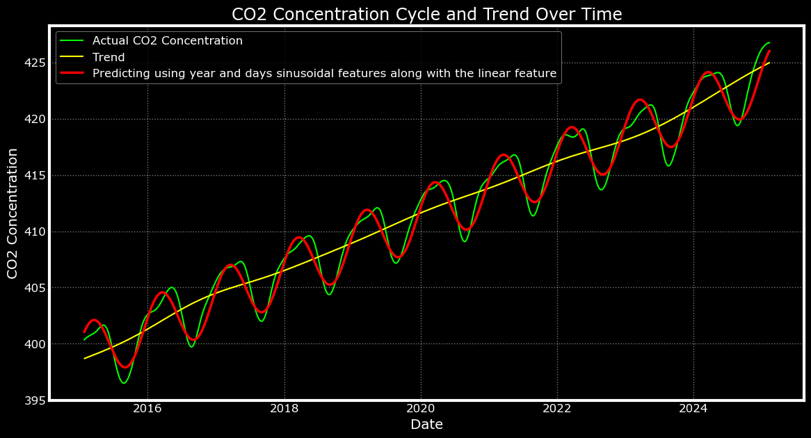
1y_pred = model_7.predict(X_sin_cos_day_year)
2plot_predictions(y_pred, 'Predicting using year and days sinusoidal features along with the linear feature')

When Simplicity Meets Structure: The Final Fit

The strategic simplification paid off beautifully. By removing the noisy month-based sine and cosine features, reintroducing the number of days as a linear trend component, and restoring a second hidden layer with ReLU activation, the model achieved what can only be described as a near-perfect fit.

The red prediction line now tracks the actual CO₂ concentrations (green line) with remarkable precision across the entire time series. Most importantly, the model has learned to combine both temporal components: the smooth seasonal oscillations are preserved with accurate amplitude and timing, while the steady upward trend — represented by the yellow trend line — is closely followed.

Gone are the jittery, noisy predictions from earlier iterations. In their place are clean, smooth curves that respect both the cyclical nature of seasonal CO₂ variations and the underlying long-term increase in atmospheric concentrations. The predictions now oscillate seamlessly along the rising trend, illustrating just how powerful a well-balanced model can be.

This result is a testament to the idea that modeling complex time series doesn’t always require more sophisticated algorithms — sometimes, the key lies in thoughtful feature selection and an architecture that is just expressive enough. By retaining the sine and cosine of day and year to model seasonality, adding a linear trend proxy via the day count, and keeping the model lightweight with a two-layer structure, I was able to capture the essential dynamics of the system with surprising clarity.

Final Thoughts: Lessons in Modeling Cyclical and Trending Time Series

This experiment began as a casual challenge and evolved into a deeply satisfying exploration of how to model complex time series data using relatively simple neural networks. Along the way, I was reminded that success in machine learning doesn’t always come from bigger models or fancier algorithms — it often comes from understanding the data, and engineering the right features to express what the model should learn.

By progressively iterating through architectural tweaks and feature combinations, I uncovered a compact solution that captures both the cyclical seasonality and the long-term upward trend of atmospheric CO₂ concentrations. The final model — powered by just a few well-chosen features (sine and cosine of day and year, and a linear time index) and a two-layer neural network — proved that small, intuitive models can go a long way when guided by the right inputs.

The key takeaway? When working with time series data that exhibits both cyclical patterns and trends, start with your intuition. Decompose the signal, understand its components, and design your features to mirror the phenomena you're trying to model. Sometimes, the smartest thing you can do is make the data speak more clearly — and let a simple model do the rest.

Try It Yourself — and Share Back!

If you've ever struggled with time series data that mixes cycles and trends, I hope this walkthrough sparked some ideas for your own experiments. Try applying this approach to your own datasets — tweak the features, play with architectures, and see what insights emerge. You might be surprised by how far a simple model can go with the right inputs.

I'd love to hear what you discover! If you’ve tried a variation of this experiment, have questions, or want to share your results, feel free to drop a comment, reach out, or connect. I’m always excited to learn from others who are exploring creative ways to model complex patterns in time.

Let’s keep learning together.